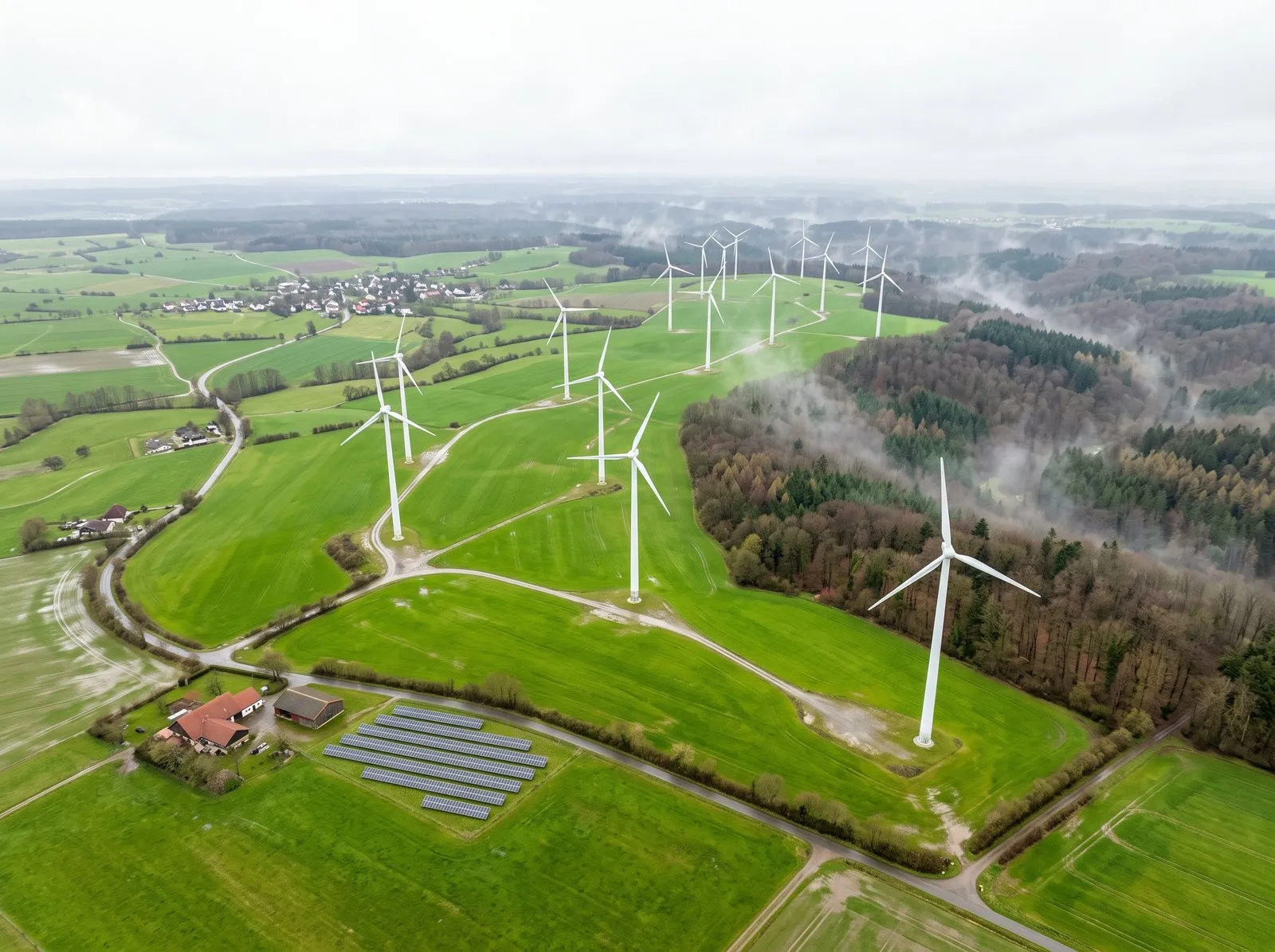
Onshore and offshore wind convert the same weather resource into electricity, but their operating environments differ. Terrain, coastal conditions, turbine layouts, maintenance access and grid connections influence production. Neither setting provides constant power: offshore wind can also experience low-wind periods, storms and operational constraints. Forecasting helps translate changing conditions into an expected generation profile.
Wind speed is only the beginning
A turbine's power response is nonlinear. Output depends on the operating range, air density and control behaviour as well as wind speed. Turbine-height conditions can differ from a nearby weather observation or model grid value. Plant-level estimates also need to account for the collection of turbines rather than multiplying one idealised power curve by the turbine count.
Layouts and wakes matter
Upstream turbines alter the flow reaching turbines behind them. The effect changes with wind direction and atmospheric conditions. A wind farm's history can help identify its aggregate behaviour, but equipment changes and operating restrictions need to be recorded. Weather-to-power conversion should be tested for the actual plant rather than assumed transferable without adjustment.
Operational availability changes feed-in
Maintenance, outages, grid restrictions and site-specific environmental conditions can reduce production. Offshore access can depend on weather and logistics, but an energy forecast does not by itself establish a safe maintenance window. Distinguish potential generation from expected exported power and agree which availability information is supplied.
Different horizons support different decisions
Day-ahead forecasts help prepare schedules and trading positions. Intraday updates incorporate newer information as the delivery period approaches. Longer-horizon estimates can inform planning, but uncertainty increases and the decision context changes. Compare forecasts at equal issue times and deadlines. A later update should not be presented as the result available to an earlier decision.
Evaluate a representative portfolio
Measure errors on a consistent basis, inspect seasonal and site differences, and include a baseline. Aggregating sites can partly cancel local errors, while large-scale weather events can affect many plants together. Historical capacity figures from the original 2016 article describe its publication period and have been removed from this evergreen explanation. The forecasting requirement remains: connect weather, plant characteristics and availability to a verifiable operational result.
Interpreting a power curve
A manufacturer’s power curve describes output under defined conditions. Real farm output also reflects wakes, availability and local flow. A forecast model may use that curve as a starting point, but it should not be treated as a complete representation of exported power. Changes in turbine control or plant configuration should be recorded because they can alter the measured relationship.
Weather diversity and shared risk
Different locations can reduce some local variability when combined in a portfolio. However, a large weather system can produce related errors across many sites. A portfolio forecast should use consistent issue times and asset definitions, and an uncertainty assessment should consider those relationships. Simply adding independent site margins may misrepresent the aggregate risk.
What to provide for an evaluation
Prepare a stable asset list, capacity definitions, generation observations and known availability events. Agree whether the forecast covers weather-dependent potential or actual expected feed-in. Fix the scheduling deadline and compare the information available then. Inspect ramps, low-output periods and high-output conditions as well as the overall error. Those checks connect an explanation of wind technology with the operational evidence an operator or trader needs to choose a forecasting service.